What does the XLOOKUP function do?
To learn how to use the XLOOKUPXLOOKUP function is a powerful alternative to VLOOKUP, HLOOKUP, and INDEX MATCH. It allows you to search for a value in a range and return a corresponding value from another range. Unlike VLOOKUP, it works both vertically and horizontally, and it doesn’t require the lookup column to be the first column in the range.
What are the advantages of using the XLOOKUP function?
The XLOOKUP function is a kind of improved and merged version of VLOOKUP and HLOOKUP. It comes as a strong replacement for those two functions and has many advantages when working on datasets such as:
- No need for column index numbers – Unlike
VLOOKUP, which requires specifying a column number,XLOOKUPdirectly references the return column. - Works with both vertical and horizontal lookups – Replaces both
VLOOKUPandHLOOKUP. - Handles missing values – The
[if_not_found]argument prevents errors if a value isn’t found. - Supports wildcard matches – Useful for partial searches.
- Can search in reverse order – Helps when searching for the last occurrence.
How to use the XLOOKUP function in Excel?
Syntax of XLOOKUP
=XLOOKUP(lookup_value, lookup_array, return_array, [if_not_found], [match_mode], [search_mode])- lookup_value – The value to search for.
- lookup_array – The range where the lookup value is found.
- return_array – The range from which to return a corresponding value.
- [if_not_found] (Optional) – Value returned if the lookup value isn’t found.
- [match_mode] (Optional) – Specifies exact or approximate match:
- 0 (default): Exact match
- -1: Exact or next smaller value
- 1: Exact or next larger value
- 2: Wildcard match
- [search_mode] (Optional) – Defines search direction:
- 1 (default): Search from first to last
- -1: Search from last to first
Examples of XLOOKUP usage
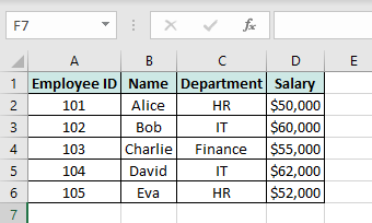
Let’s take the following table as an example. This table consist of fictional employee data and has 4 columns which are Employee ID, Name, Department, Salary.
| A | B | C | D | |
|---|---|---|---|---|
| 1 | Employee ID | Name | Department | Salary |
| 2 | 101 | Alice | HR | $50,000 |
| 3 | 102 | Bob | IT | $60,000 |
| 4 | 103 | Charlie | Finance | $55,000 |
| 5 | 104 | David | IT | $62,000 |
| 6 | 105 | Eva | HR | $52,000 |
1. How to find an Employee’s Salary by Name
If you want to find Bob’s salary, use:
=XLOOKUP("Bob", B2:B6, D2:D6, "Not Found")➡️ Returns $60,000
2. How to find an Employee’s Department by ID
If you want to find the department of Employee ID 104, use:
=XLOOKUP(104, A2:A6, C2:C6, "Not Found")➡️ Returns "IT"
3. How to find the Last Employee in IT
If you want to find the last IT employee’s name:
=XLOOKUP("IT", C2:C6, B2:B6, "Not Found", 0, -1)➡️ Returns "David"
Advanced Examples of XLOOKUP usage in Excel
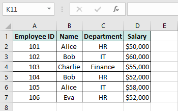
When searching for values based on multiple conditions (e.g., finding an employee’s salary based on both name and department), XLOOKUP alone won’t work directly. However, you can combine multiple criteria using a helper column or an array formula. Let’s use a similar table to the previous one:
| A | B | C | D | |
|---|---|---|---|---|
| 1 | Employee ID | Name | Department | Salary |
| 2 | 101 | Alice | HR | $50,000 |
| 3 | 102 | Bob | IT | $60,000 |
| 4 | 103 | Charlie | Finance | $55,000 |
| 5 | 104 | Bob | HR | $52,000 |
| 6 | 105 | Alice | IT | $58,000 |
| 7 | 106 | Eva | HR | $52,000 |
1. Find an Employee’s Salary Based on Name AND Department
If we want to find the salary of "Bob" in the "HR" department, we need to match both name and department.
📌 Formula (Array Formula Approach)
=XLOOKUP(1, (B2:B7="Bob") * (C2:C7="HR"), D2:D7, "Not Found")Explanation:
(B2:B7="Bob")creates an array of TRUE (1) or FALSE (0) where Bob appears.(C2:C7="HR")does the same for the department.- Multiplying them (
*) ensures only rows where both conditions are met return1. XLOOKUP(1, …, D2:D7, "Not Found")finds the first row where both match and returns the salary.
➡️ Result: $52,000 (Bob in HR)
2. Find the Latest Salary Entry for a Given Name
If we want to find the most recent salary recorded for "Alice", we need to search from bottom to top.
📌 Formula (Reverse Search Mode)
=XLOOKUP("Alice", B2:B7, D2:D7, "Not Found", 0, -1)- This searches for
"Alice"but in reverse order (-1insearch_mode), ensuring the latest entry is returned.
➡️ Result: $58,000 (Alice in IT)
3. Find an Employee’s Salary Based on Name AND Partial Department Name
If we don’t know the exact department but know part of it (e.g., "Fin" for "Finance"), we can use wildcards.
📌 Formula (Wildcard Matching)
=XLOOKUP(1, (B2:B7="Charlie") * ISNUMBER(SEARCH("Fin", C2:C7)), D2:D7, "Not Found")SEARCH("Fin", C2:C7)checks if"Fin"appears anywhere in the department column and return its position inside the string where it was found.ISNUMBER(SEARCH(…))converts it into TRUE/FALSE (1/0).- The rest works like our multiple criteria example.
➡️ Result: $55,000 (Charlie in Finance)
4. Find the Most Recent Entry for a Department
If we want the latest salary recorded in the "IT" department:
📌 Formula
=XLOOKUP(1, (C2:C7="IT"), D2:D7, "Not Found", 0, -1)➡️ Result: $58,000 (Alice in IT)
See also our products and tools
Gumroad Shop: