How to dynamically change chart types in Excel?

Why dynamically change chart types in Excel can be useful

Learning to dynamically change chart types in Excel may seem like a niche skill, but it can actually save your design — and your sanity — in specific situations.

Choosing the right chart type is crucial because it directly impacts how your data is perceived, understood, and acted upon. For static, well-defined datasets, selecting a chart type is typically a one-time decision during the workbook setup. However, things change when you’re dealing with dynamic data that evolves over time.

In these cases, a chart type that initially made perfect sense might no longer be appropriate. For example, a radar chart requires a minimum number of data points to display correctly. If your dataset temporarily lacks those points, the chart becomes unreadable or visually broken. Being able to switch to another chart type — say, a bar chart — until your data grows back to the right size can be incredibly useful.

Why can’t I find this feature in Excel?

For reasons not well explained by Microsoft, Excel doesn’t natively offer a built-in feature to dynamically change chart types in Excel based on conditions or formulas.

To be fair, most beginner or intermediate users rarely encounter the need for this. However, if you’re working on interactive dashboards or automated reporting, this feature becomes extremely relevant.

Luckily, there’s a workaround — and it’s simpler than it sounds.

Step-by-step Method to dynamically change chart types in Excel

This method is easy to follow, but precision matters, especially when dealing with sizes and placements.

⚠ You will also need to prepare a small image file for this trick

The image itself won’t be visible, but Excel needs it as a placeholder. Any image format should work, but JPEG or PNG is recommended.

Step 1: Prepare your dataset

Start by organizing your dataset to reflect real use cases. This helps identify structural issues early.

Use an Excel table (Ctrl + T) to ensure proper dynamic handling when rows are added or removed.

Step 2: Create your charts

Next, create each chart type you want to switch between. All charts should use the same dataset as a source.

Since these charts aren’t meant to be seen directly by users, place them in a separate worksheet tab — you can hide this sheet later.

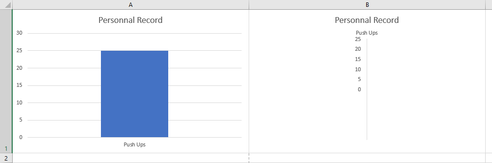
In this example, we’ll use a bar chart and a radar chart.

Step 3: Insert the prepared image

We should now have a proper dataset and the charts ready. It’s time to insert the image we previously prepared. To insert an image from your computer to an Excel workbook go to:

Insert > Pictures > This Device

Once inserted, position the image exactly where you want the dynamic chart to appear. Don’t worry about what the image shows — it won’t be visible to the user. It will be replaced by a chart via formula.

Step 4: Link the charts to the image

Now for the clever part: we’ll use the image to display the correct chart based on a condition.

✅ A. Prepare the chart layout

• Go to the sheet with your charts.
• Place each chart into its own dedicated cell, and match the chart size to the cell size.

⚠ Excel automatically resizes charts when rows or columns they are overlapping with change. To avoid misalignment, make sure there are no overlaps between the rows and columns of the cells you plan to use and the charts.

Matching both sizes can either be done manually (less accurate) or by comparing the exact charts’ size (available in the chart formatting options) and the cells’ size (the cell size can be confirmed when using View > Page Layout and right clicking on the row or column then row height/column width).

The second method seems more accurate but could still has issues as it seems there are sometimes mismatches between both the cell and chart dimensions even when manually inputting the same width and height as numbers.

The most reliable approach:

• First adjust the cell dimensions slightly larger than needed.
• Then insert the chart into the cell and resize it manually to match the cell exactly.
• Use a consistent layout (e.g., all charts in the same row) to simplify alignment.
• Once the first chart is fitted to its cell, match the second cell dimensions based on the first one.

✅ B. Define the chart selection criteria

We’ll now create the logic to determine which chart to show based on the data.

One problem: Excel doesn’t seem to be able to apply complex direct references and calculations on an image unless the formula is defined via the Name Manager.

Trying to directly input the formula as a source for the image would trigger the following error message:

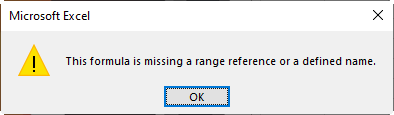
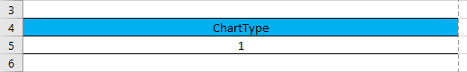
First, let’s prepare the main criteria. In our example, we’ve used a simple bar chart and a radar chart. A radar chart requires a minimum of 3 data points to display correctly. We need to count the number of exercises available in our dataset. Once the number reaches 3 we can switch from the bar chart to the radar chart. In a helper cell (e.g., Charts!A5), enter:

=COUNTA(PR_Tracker[Exercise])

✨Here PR_Tracker is the table name and Exercise the table column where the exercises names are inputted.

⚠ This can also be done directly in the Name Manager but we chose to use a helper cell for simplicity.

✅ C. Create the final formula in Name Manager

The Name Manager can be found under:

Formulas > Name Manager

Open the Name Manager -> Click New.

• Choose a Name for the formula in the Name textbox (e.g., ChangingChart)
• Go to the Refers to textbox to input the final formula.

In our case, as our criteria formula was inputted in the helper cell A5, we need to refer to it in the final formula:

=IF(Charts!$A$5<3,Charts!$A$1,Charts!$B$1)

Here, A1 and B1 refer to the cells containing the bar and radar charts, respectively.

Then press Ok and Close.

✅ D. Link the formula to the image

If you reached this step you're almost done. Return to the main worksheet where your image is. Select the image, then click into the formula bar and type:

=ChangingChart

Hit Enter. If all is set up correctly, your image will now transform into the appropriate chart depending on your data.

Test your condition (in this example, change the number of exercises) and watch the chart type update accordingly.

✅ Final thoughts

This method allows you to dynamically change chart types in Excel even though Excel doesn’t support it natively. It's a clever trick that’s both flexible and scalable.

Let us know if this helped you — or if you'd like more tips like this!