How to freeze rows and columns in Excel?

What does the Freeze panes feature do?

In this article, we’ll show you how to freeze rows and columns in excel. In Excel, “Freeze Panes” is a feature that allows users to lock specific rows or columns. Locked columns and rows remain visible while scrolling through the worksheet. This is especially useful when working with large datasets where headers or key reference columns need to stay in place for easy readability

To summarize its advantages:

• Keeps headers visible – Ensures column titles stay at the top of the screen while scrolling down.
• Locks important reference columns – Keeps key data (e.g., names, IDs) visible when scrolling sideways.
• Enhances data analysis – Makes it easier to compare data across rows and columns without losing context.
• Improves navigation – Helps in efficiently working with large datasets by reducing the need to scroll back.

How to Use “Freeze Panes” in Excel

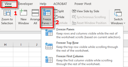
• Go to the View tab.
• Click Freeze Panes

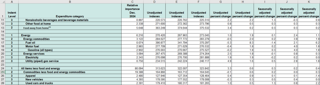
Freeze the top row

• Click Freeze Panes→ Freeze Top Row (keeps the first row visible).

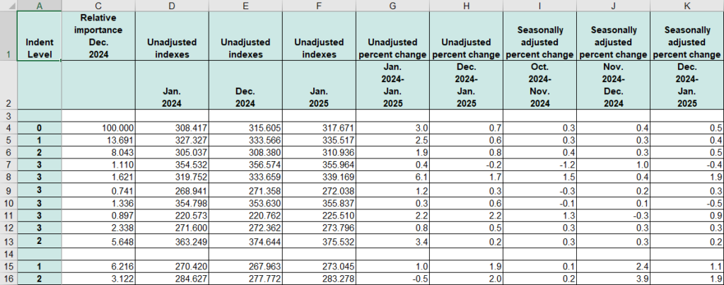
Freeze the first column

• Click Freeze Panes → Freeze First Column (locks the first column).

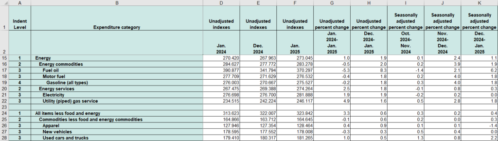
Freeze multiple rows and columns

• Select the cell below the rows and to the right of the columns you want to freeze.
• Go to View → Freeze Panes → Freeze Panes.